---

The Mathematical Predictive Model

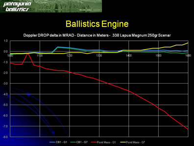
The ballistics engine of ColdBore© is a propietary aeroballistics model based on a Kalman modified filter, which includes numerous proprietary extensions. The only resemblance to the method developed by the late Professor Arthur J. Pejsa ( who finished his research circa 1953 ) is just partially related to the way it handles the drag slope. This propietary method has no velocity or range restrictions, covering the full spectrum from supersonic, transonic and subsonic trajectories at extended ranges with muzzle velocities starting at any sonic boundary, giving a continuous, non-linear solution. This engine is the result of over 3 years of original research in the field of aeroballistics.

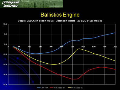
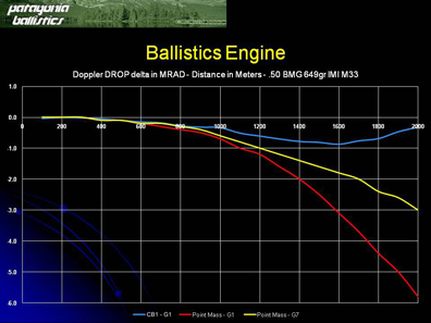
It has been proved time after time its superior predictive capability over the traditional "Point Mass" method that is used on almost any other program, that requires the use of the G7 drag function to yield reasonable solutions in and beyond the transonic range. Even using G7 the results may be not satisfactory, usually calling for the so called "custom drag curves" and the use of "truing" procedures. None of these shortcomings are needed in ColdBore© to produce outstanding predictions.

Many enhancements to the algorithms were developed, using both iterative and recursion approaches to solve the problem of computing downrange figures for velocity, time of flight and drop, the main variables of the solution from which others parameters are derived.

The model is an analytic, closed-form solution that doesn’t use tables generated for standard-shaped projectiles, a fact of paramount importance, since while it does not rely on the G1/G7 drag model used in most of the available programs, (some following the Mayeveski-Ingalls tables), the present method can use a readily available, G1/G7 ballistic coefficient as published, incorporating a custom drag function in order to model the specific projectile.

Since it effectively uses an analytic function ( of Mach number ) in order to match the drag curve of the specific bullet, it does not need to rely on other drag tables to approximate a better fit.

A ballistics software foundation rests in its ability to predict accurate trajectories, matching field results as the ultimate test.

Nearly all ballistic software take for granted that a specific drag function correctly describes the drag characteristics of a bullet as related to its ballistics coefficient, consequently, whether the bullet style is a flat-based, spitzer, a boat-tail, ULD, etc they take care of them to the same drag function as indicated by the published BC, usually the G1/G7 function.

The state of the art mathematical approach taken here, is quite different and a major improvement, of special application to the long range shooter.

Being practical, the use of the published BCs data as available, by almost every major bullet manufacturer is almost mandatory. However this program does not use it to calculate the changes to the drag function over the supersonic velocity range.  In other words, this program ballistics engine uses a drag coefficient (DC) that affects the calculated rate of bullet deceleration.

Applying this DC, the resultant trajectory calculations are very accurate for that particular bullet because the drag function has effectively been tailored for that particular bullet.

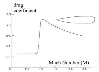
As the drag coefficient can be modeled as a simple function of the Mach number, the particular functional form of the drag coefficient allows variations in the shape of the drag curve to be considered parametrically.

It's easily demonstrated that the projectile trajectory and velocity history can be characterized in terms of three parameters: the projectile’s muzzle velocity, a parameter related to the muzzle retardation, and a single parameter defining the shape of the drag curve.

Other approaches ( on the market ) base their predictions on trying to make a match of a specific bullet ( yours ) to like drag data which is available to examine the variation of the drag coefficient with Mach number in the standard axisymmetric ( having symmetry around an axis ) projectile shapes, that were tested in the early to mid-1900’s.

These resulting drag curves are referred to as the Ingalls, G1, G2, G5, G6, G7, and G8 drag curves.

Most bullet manufacturers assume and publish the G1 drag function shape. Examination of the form of a G1 standard-projectile, will to the obvious conclusion that it doesn't apply to the modern boattail bullet shapes in common use today. The G7 or G8 shape is much more appropriate but general availability of these ballistic coefficients is almost nonexistent.

Particularly, the G1, G5, and G7 curves model a specific bullet form, since they were deduced from, and it's common for some programs to adapt ( modify ) the G1 drag curve in an effort to fit the G5 to G7 bullet shapes, and in other words, these approaches are, at best an improvement to model modern bullet shapes in order to make predictions more accurate.

That's why the BC must be defined as a function of velocity. The present solution uses the actual drag, and not rely on an average fit to a non-representative standard or table-based drag function.

In short, what these models can, is to compute accurate trajectory values if range is moderate, up to approximately 600 yards, beyond that, you need a different way to model air drag and to account specifically for a drag curve that matches your bullet dynamics. This is what this method does precisely.

The method used here takes on a different approach, since if the shooter takes the necessary effort to actually measure the Drag Coefficient, the model will make an almost perfect fit, under different environmental conditions, thus yielding very precise downrage values for Velocity, Time of Flight and Drop.

The key element to compute accurate trajectories is the Drag curve, and of course its modeling via an appropriate function.

To accomplish this we need to know its initial values, its mean value and its maximum value, all across the supersonic, transonic and subsonic range or at any initial Velocity if not starting at typical rifle's velocities.

These aspects of the drag curve are modeled through a retardation factor <b>F</b>, or its inverse the deceleration A,  slope factor ( the Drag Coefficient ) N, which is the rate of change of the retardation with range, and finally, the velocity at which the curve changes Vk, having reached its maximum value.

For the sake of simplicity and with the design criteria of being practical, the user only needs to deal with the slope factor, and that coupled with the G1-based BCs will yield very accurate results, so there is no need, at this level, to cope with velocities boundaries, since they are in fact modeled by the program itself, as well as the necessary different slope factors needed when the bullet's velocity goes through different sonic ranges.

Typically, this slope factor goes, in terms of bullet shape, from 0.1 ( flat-nose ) to 0.9 ( very-low-drag ), and a default value of 0.5 can be used for most modern spitzer-type bullets with confidence, and if not possible to obtain it from actual measurements, its value can be determined from bullet's shape.

However for maximum accuracy, especially at long range, its value should be determined by the method used here, which involves the measurement of four velocities ( loss ), that evaluate retardation <b>F, ( Fa and Fb )</b> at two known apart distances.

Do not confuse BCs with this drag value, since two bullets with the same BC may have different deceleration ratios, due to shape, materials, construction, barrel's twist rate, etc.

WARNING: It's important to remark, that this program does not favor any other method to evaluate it, especially those based on measuring Drop at a certain range, because there are so many errors that can be introduced it doesn't lend itself as being very viable. Its determination is totally affected by shooter/gun errors and in fact does not represent the actual problem of velocity, which can be measured very precisely by means which are both available and affordable.

One of the most frequently asked questions is "how accurate are the calculated downrange values?"

As with any software with a good mathematical model, the accuracy of the input values determines the accuracy of the output values.

In exterior ballistics, elements such as shape, caliber, weight, initial velocities, rotation, air resistance, and gravity help determine the path of a projectile from the time it leaves the gun until it reaches the target.

While the accuracy of the mathematical model is superior, bare in mind that actual field results can differ due to the shooter's ability, the gun, the ammo and a myriad of other factors that affect a bullet's flight, making necessary an inordinate amount of time and equipment to collect, thus rendering impossible a practical solution, especially at longer ranges.

At the same time, there are too many variables that magnify their effect at such ranges, not to mention the shooter's ability to cope with such a challenge.

On the other hand, as any shooter ( especially those involved in long range engagements ) know, some effects like wind are difficult to estimate, or the individual characteristics of a rifle for example, or plain shooter errors, will make differences between actual impact location versus predicted ones more evident. Unfortunately there is no practical way to cope or account for these changes, and eventually nothing replaces carefully collected field data.

The most common ballistic error sources are variations of the muzzle velocity, variations of the angle of departure and the azimuth, variations of the bullet drag, variations of wind speed and wind direction, variations of the lift force, bullet static and dynamic unbalances, etc and from the shooter's side we can count on aiming errors, sighting error, canting of the gun, etc.

It's important to note that predicting accurate downrange values past the 3000 yards/meters limit, is almost impossible without taking special, ad-hoc efforts well beyond the scope of most shooters. A good example as well as a main source for errors are the published BC values that we must rely on and take for granted.

So, if the input values are as accurate as can be practically determined, then there won't be any statistically significant difference between the calculated down range values and actual measured values, within the range of values allowed for both input data as well as it's ouput.

If you know anything about statistics, then you know that any given shot may not match the calculated value, but the average of a group of shots comes very close, and the more shots in the group, the closer the true average is to the calculated value. The difference between individual shots and the group's average is called Variability.

However, it should be recognized, , that neither aiming errors nor the ballistic dispersion can ever be reduced to zero, and therefore whether or not a target will be hit by any particular shot is a question of probabilities, depending on the size of the target, the proficiency of the rifleman, the accuracy of the information about the conditions under which the shot will be made, and the ballistic dispersion of the gun/ammunition system.

The gun enthusiast should learn by experience and recognize realistically the outer limits of the ranges at which various types of targets can be engaged with a reasonable probability of success.

Exterior ballistics refers to the trajectory of a bullet once it has left the muzzle of a firearm.

Exterior ballistics is a generic term used to describe a number of natural phenomena that tend to cause a bullet in flight to change direction or velocity or both. These phenomena are gravity, drag, wind, drift (when considering spin-stabilized bullets) and Coriolis effect.

The computation of relative-motion effect produces the actual point of collision between the bullet and the target. The computation of the effects of ballistics produces aiming corrections as a result of the curvature of the bullet's flight path.

These corrections don't change the final collision point, but cause the trajectory of the bullet to intersect the flight path of the target. The ultimate aim of ballistic computation, then, is to produce angular corrections to the azimuth and elevation values derived from the relative-motion results.

Inherent in these calculations is the computation of time-of-flight of the bullet, which in turn is used to facilitate the relative-motion computation.

Ideally, it is desired to produce a procedure that totally describes the complex trajectory of a bullet. When provided the coordinates of the future target position as input data, this procedure would produce angles of launch and bullet time-of-flight as output.

It must be emphasized here that the central problem of bullet delivery is the solution of the intersection of two curves, one described by the motion of the target and the other described by the motion of the bullet.

It's knowledge can be used to extend the effective range of a hunting rifle, help set sights for different locations and weather conditions, select calibers and ammunition or even help select reload components, all of this based on sound mathematical principles.

The analysis and prediction of the trajectory of projectiles has been a subject investigated for many centuries and is still a topic of interest today.

The interest and advancement of the problem has come from two fields: mathematics and physics. As a mathematical problem, the focus has been on the methods for solution of the governing equations.

Some of the most noted mathematicians and physicists of the past several centuries, such as Galileo, Bernoulli, and Euler, have investigated the mathematical solution of this problem and have obtained technical advances important for trajectory prediction.

To accurately determine the trajectory of a projectile, one must also properly account for the physical effects such as gravity and the air resistance or drag of the projectile. In additional to his laws of motion, Newton has also been credited for the development of the quadratic law of resistance characterizing the aerodynamic drag of a body.

Further advances have shown that more sophisticated characterization of the drag is required to predict the trajectory across the complete flight regime of many projectiles.

Over a century ago, Mayevski found that it was possible to express the drag of a projectile as proportional to a power of the velocity within restricted velocity regimes. This has been described as the Mayevski Law of Resistance. Piecing together the drag in adjacent velocity regimes using this approach allowed the drag to be characterized over the complete flight regime. Mayevski’s advance led to further developments in trajectory prediction methods.

One of the more famous methods is the Siacci method. The Siacci method was widely used to predict the flat-fire trajectories for decades after its initial development. The method still has some adherents in the sporting and ammunition community.
 
With the advent of the computer, the Siacci method has been replaced by more modern numerical methods.

These methods allow rapid and accurate computation of the projectile’s trajectory provided the physical characteristics of the projectile (such as the drag) and the atmosphere are appropriately modeled. Modern aerodynamic analysis and trajectory programs provide an excellent means of accurately determining the flight behavior of specific designs.
 
The increased sophistication of trajectory prediction methods has some unfortunate consequences. The user must often provide an array of details that may or may not be relevant to the answer that is being sought. Additionally, these methods often obscure critical insights into the relationship between important parameters that produce the physical behavior of interest.

For example, there are occasions where a ballistician would like to be able to predict aspects of the flight trajectory without completely defining the geometry or aerodynamic characteristics of a projectile, such as in preliminary design or experimental testing.

In these cases, simplified analyses can provide accurate results with the minimum amount of relevant input from the user and provide the designer with a clearer understanding of the primary design variables.

The force of gravity always tends to accelerate an object downward toward the center of the earth. The effects of this force on the trajectory of a bullet are well known and if considered alone result in very simple solution to the trajectory problem.

In a vacuum on a "flat" nonrotating earth, the horizontal component of the initial velocity of the bullet (V0 x cos ) remain unchanged. However, the vertical component (V0 x sin ) is continuously changed as a result of the acceleration due to gravity. This changing vertical velocity results in a parabolic trajectory.

In the vacuum trajectory situation, the solution is easily obtained because of the simplifications and assumptions made in formulating the problem.

When the effects of the atmosphere are considered, forces other than gravity act on the bullet, which cause it to deviate from a pure parabolic path.

This deviation results specifically from the dissipation of energy as the bullet makes contact with the atmosphere.

It has been found that the loss of energy of a projectile in flight is due to :

- Creation of air waves--The magnitude of this effect is influenced by the form (shape) of the bullet as well as by the cross-sectional area.

- Creation of suction and eddy currents--This phenomenon is chiefly the result of the form of the bullet and in gun projectiles specifically, the form of the after body.

- Formation of heat, thus energy is dissipated as a result of friction between the bullet and the air mass.

The combined effect of energy loss is a deceleration of the projectile during its time-of-flight. This deceleration acts to decrease the velocity of the bullet as it travels through the atmosphere. For a given projectile form, the retardation in velocity is directly proportional to the atmospheric density and to the velocity itself. This deceleration is called parasitic drag.

Parasitic drag always acts in a direction opposite to that of the motion of the bullet.

As a result, two fundamental interdependent actions take place while a bullet is in flight.

First, the force of drag at any point in the bullet's trajectory is a direct function of the velocity at that point. Because the drag force is continuously retarding the velocity of the bullet, the force of drag itself is continuously changing over the entire time-of-flight of the bullet, with drag dependent upon velocity and in turn velocity dependent upon drag.

Thus, the magnitude of both the velocity and the drag are changing with each dependent upon the other. Second, as the bullet travels the curved path of the trajectory, the angle is never constant, which results in the force of drag continuously changing direction throughout the entire flight of the bullet.

The force of drag constantly changes in magnitude as a function of velocity and in direction as a function of the direction of motion of the bullet.

The end result of drag is to slow the projectile over its entire trajectory, producing a range that is significantly shorter than that which is achievable in a vacuum.

While the vacuum trajectory is symmetric about the mid-range value, with the angle of fall equaling the angle of departure, the atmospheric trajectory is asymmetric. The summit of the trajectory is farther than mid-range, and the angle of fall is greater than the angle of departure.

Additionally, the atmospheric trajectory is dependent on projectile mass due to external forces--which also, unlike the vacuum case, causes the atmospheric trajectory's horizontal component of velocity to decrease along the flight path. This results in a computation of the necessary departure angle to affect maximum range, whereas in a vacuum the maximum range's departure angle is 45°.

In consideration of the elevation at which maximum range is achieved, there are two offsetting effects: the change in drag with projectile velocity and the atmospheric density. A projectile's velocity is greatest immediately upon leaving the gun, thus drag is greatest at this time also.

For small, lightweight projectiles, deceleration is greatest at the beginning of flight; therefore, to take advantage of improvement in horizontal range while the velocity is greatest, it is necessary to shoot at elevations less than 45°.

In large projectiles such as those employed on battleships it is best to employ elevations above 45° to enable the projectiles to quickly reach high altitudes where air density and thus drag are decreased. Range increases result from the approximation of vacuum trajectory conditions in the high-altitude phase of projectile flight.

The effects of wind can be divided into two components: range wind and cross wind. Range wind is that component of wind that acts in the plane of the line of fire. It serves to either retard or aid the projectile velocity, thus either increasing or decreasing range.

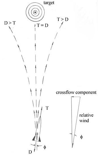
Cross wind acts in a plane perpendicular to the line of fire and serves to deflect the projectile either to the right or left of the line of fire.

Wind acts on the projectile throughout the time of flight; therefore, the total deviation in range and azimuth is a function of the time-of-flight.

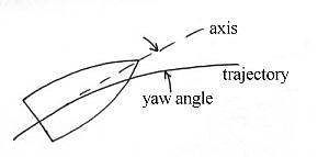
Drift of a gun projectile is defined as the lateral displacement of the projectile from the original plane of fire due only to the effect of the rotation of the projectile. The principal cause of the drift lies in the gyroscopic properties of the spinning projectile. According to the laws of the gyroscope, the projectile seeks, first of all, to maintain its axis in the direction of its line of departure from the gun.

The center of gravity of the projectile, however, follows the curved path of the trajectory, and the instantaneous direction of its motion, at any point, is that of the tangent to the trajectory at that point. Therefore, the projectile's tendency to maintain the original direction of its axis soon results in leaving this axis pointed slightly above the tangent to the trajectory.

The force of the air resistance opposed to the flight of the projectile is then applied against its underside.

This force tends to push the nose of the projectile up, upending it. However, because of the gyroscopic stabilization, this force results in the nose of the projectile going to the right when viewed from above.

The movement of the nose of the projectile to the right then produces air resistance forces tending to rotate the projectile clockwise when viewed from above. However, again because of the gyroscopic stabilization, this force results in the nose of the projectile rotating down, which then tends to decrease the first upending force.

Thus, the projectile curves or drifts to the right as it goes toward the target. This effect can easily be shown with a gyroscope.

A more detailed analysis of gyroscopic stability would show that a projectile is statically unstable, but because of the gyroscopic effects, becomes dynamically stable. These effects actually cause the axis of the projectile to make oscillatory nutations about its flight path. Also the Magnus Effect, where a rotating body creates lift (figure 20-9) must be considered. The Magnus Effect is what causes a pitched baseball to curve.

The preceding effects have all considered the earth to be flat and non-rotating.

The Coriolis effect is caused by the rotation of the earth.

The Coriolis effect is an inertial force described by the 19th-century French mathematician Gustave Gaspard Coriolis in 1835.

Coriolis showed that, if the ordinary Newtonian laws of motion of bodies are to be used in a rotating frame of reference, an inertial force ( acting to the right of the direction of body motion for counterclockwise rotation of the reference frame or to the left for clockwise rotation ) must be accounted for in the equations of motion.

The effect of the Coriolis force is an apparent deflection ( and it's also called a fictitious force ) of the path of an object that moves within a rotating coordinate system.

The moving object does not actually deviate from its path, but it appears to do so because of the motion of the coordinate system. While the effect of the earth's movement while a projectile is in flight is negligible for short and medium range shots, for longer range shots the Coriolis effect may cause the projectile to drift considerably from it's intended trajectory.

Actually this is not the case, and centripetal acceleration and Coriolis acceleration caused by the rotating earth must be considered. The centripetal acceleration of a point on the earth's surface will vary with its distance from the rotation axis. Thus, the difference in the velocities of the launcher and the target because of their different locations on the earth's surface must be considered.

The Coriolis acceleration force is created when a body or projectile moves along a radius from the axis of rotation of the earth ( or a component of it ).

This force tends to curve an object to the right in the Northern Hemisphere and to the left in the Southern Hemisphere. An observable example would be that the air moving outward from a high becomes clockwise wind and air moving into a low becomes counterclockwise wind.

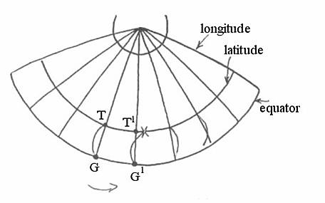
In the Northern Hemisphere the deflection is to the right of the motion; in the Southern Hemisphere it is to the left. The Coriolis deflection of a body moving toward the north or south results from the fact that the earth's surface is rotating eastward at greater speed near the equator than near the poles, since a point on the equator traces out a larger circle per day than a point on another latitude nearer either pole.

A body traveling toward the equator with the slower rotational speed of higher latitudes tends to fall behind or veer to the west relative to the more rapidly rotating earth below it at lower latitudes.

Similarly, a body traveling toward either pole veers eastward because it retains the greater eastward rotational speed of the lower latitudes as it passes over the more slowly rotating earth closer to the pole. It is extremely important to account for the Coriolis effect when considering projectile trajectories, terrestrial wind systems, and ocean currents.

---